How LLMs Simplify and Improve Model Validation in Banking
The views and opinions expressed in this post are solely my own and do not necessarily reflect those of my employer. This content is for general informational purposes only and does not constitute professional advice.
- Model Validation in banking
- SR 11-7
- A Sample Model to Validate
- Reviewing the Code with an LLM
- Validation Tests with LLMs
- Leveraging LLMs to Explore Model Documentation
- An App for Model Validation with LLMs
- Conclusions
Model Validation in banking
Let’s begin by clarifying what model validation means in this post. Yes, it involves ensuring that models function correctly, a broad topic in itself, but here we’ll focus on the US banking environment, where model validation also requires adhering to regulatory standards such as SR 11-7.
Before we start, let’s see what ChatGPT has to say about model validation in this context.
Response
SR 11-7
Alright, we have a base now. We understand that validating models is a regulated process guided by SR 11-7 so let’s gather some more detail on what this should be:
Response
According to SR 11-7, a comprehensive model validation should include the following key components:
- Evaluation of Conceptual Soundness: An in-depth assessment of the model’s design, theory, and logic, including underlying assumptions and methodology. This ensures that the model is appropriate for its intended purpose.
- Ongoing Monitoring: Regular checks to confirm that the model’s performance aligns with expectations over time. This includes tracking key performance metrics and reviewing outcomes to identify any significant deviations.
- Outcomes Analysis: A quantitative comparison of the model’s predictions against actual outcomes. This step helps assess the accuracy and reliability of the model in real-world conditions.
- Benchmarking and Back-Testing: Comparing the model’s results with alternative models and validating performance through back-testing with historical data.
- Assessment of Limitations and Uncertainty: Identifying potential limitations in the model’s framework and quantifying any associated uncertainties or risks.
These elements ensure a robust validation process, enabling institutions to identify and mitigate model risks effectively, maintaining compliance with regulatory requirements.
And what form and structure does a model validation take?
Response
Model validation results, in line with SR 11-7, should be presented in a structured, transparent, and comprehensive report, typically covering the following sections:
- Executive Summary: A concise overview of the validation’s key findings, model strengths and weaknesses, and an overall assessment of the model’s risk level and validation outcome (e.g., approved, approved with conditions, or not approved).
- Scope and Objectives: A clear outline of the validation’s purpose, including the model’s intended use, its assumptions, and limitations. It should specify the validation scope, such as whether it’s a full-scope or targeted validation.
- Methodology and Approach: A description of the validation process, including the methods, tools, and benchmarks used. This part should clarify how the validation aligns with regulatory requirements and internal policies.
- Evaluation of Conceptual Soundness: Findings on the model’s design, methodology, assumptions, and overall soundness. This section often includes a detailed review of data sources, model components, and theoretical foundations.
- Ongoing Monitoring and Performance Review: Insights into the model’s stability, accuracy, and predictive power over time, along with performance metrics and any monitoring results that highlight trends or areas of concern.
- Outcomes Analysis and Back-Testing Results: Results of outcome analysis, including back-testing findings that compare predicted versus actual results. This section should provide quantitative and qualitative analyses, highlighting any discrepancies and their implications.
- Issues and Recommendations: Identification of any issues, weaknesses, or limitations, along with prioritized recommendations for improvements. This can include both short-term remediation actions and longer-term improvements to address identified risks.
- Conclusion and Sign-Off: A summary of key points and the final opinion on the model’s viability, along with sign-offs from validation team members and relevant stakeholders.
- Supporting Documentation: Additional materials such as data sources, code, validation testing details, and other relevant documents to ensure transparency and reproducibility.
Effective presentation should ensure clarity for stakeholders, including management and regulators, with visual aids like charts and tables where helpful.
In short, validating models in banking requires assessing whether they work properly and creating detailed, regulator-friendly reports. And while the process may seem simple and even obvious —and in many ways it is— it also is extremely valuable and as far as I know, not commonly adopted outside of banking. I believe other industries could benefit from a similar, standardized approach to ensure models are reliable and used appropriately through clear, consistent reporting.
Importantly, the goal of this process isn’t just to produce reports, but to improve the quality of models. And from my experience, it works. Development teams build better products when they know their work will be audited, requiring them to justify decisions and document their processes in ways that business stakeholders can easily understand.
A Sample Model to Validate
To illustrate, I’ll try to show how to validate a model and demonstrate how LLMs can help with an example.
So for this demonstration, I needed a model that resembles a real financial case. And I found this Kaggle challenge:
Home Credit - Credit Risk Model Stability.
Overview: The goal of this competition is to predict which clients are more likely to default on their loans. The evaluation will favor solutions that are stable over time.
I also discovered a working example notebook of what seems to be an example for the challenge: Home Credit 2024 Starter Notebook.
Reviewing the Code with an LLM
One initial step in model validation is a high-level code review, and LLMs can help by providing summaries, identifying issues, and offering recommendations for improvement. Below is an example of what Claude said when I asked it to summarize the code after pasting it into the interface:
Response
Let me break down this code - it appears to be implementing a credit risk or default prediction model with a focus on stability across time. Here are the key components:
- Data Loading and Preprocessing:
- Loads several CSV files containing different types of data (base tables, static data, credit bureau data, person data)
- Uses Polars (a fast DataFrame library) for initial data processing
- The data appears to be related to loan applications, with different tables containing various attributes about applicants
- Feature Engineering:
- Creates aggregated features from person-related data:
- Maximum occupation income
- Whether any applicant is self-employed
- Housing type for primary applicant
- Creates credit bureau features:
- Maximum payments overdue
- Whether payments were overdue by more than 31 days
- Creates aggregated features from person-related data:
- Model Training:
- Uses LightGBM, a gradient boosting framework
- Splits data into train (60%), validation (20%), and test (20%) sets
- Trains a binary classification model with AUC (Area Under Curve) as the metric
- Uses early stopping to prevent overfitting
- Model Evaluation:
- Calculates AUC scores for train, validation, and test sets
- Implements a custom stability metric called gini_stability that:
- Tracks model performance (Gini coefficient) across different time periods (WEEK_NUM)
- Penalizes:
- Declining performance over time (negative slope in performance)
- High variance in performance (standard deviation of residuals) * This suggests the model is being used in a production setting where stable predictions over time are important
- The hyperparameters used suggest a relatively conservative model:
- Max depth of 3
- Learning rate of 0.05
- Feature and bagging fractions < 1 for regularization
This code appears to be part of a production system where model stability over time is as important as raw predictive performance. The stability metric is particularly interesting as it penalizes both declining performance over time and high variance in performance, which are important considerations for deployed models.
It explains the code, touches on model parametrization, and highlights existing time-based performance tests. All are crucial details in a banking Model Validation.
Next, I asked for enhancements:
Response
Here are the key issues and recommended enhancements:
- Type Conversion Issues:
for df in [X_train, X_valid, X_test]:
     df = convert_strings(df)
This reassignment doesn’t modify the original dataframes. Should be:
X_train = convert_strings(X_train) X_valid = convert_strings(X_valid) X_test = convert_strings(X_test) - Missing Error Handling:
- Add error handling for file loading
- Validate data before model training
- Check for missing values
- Performance Improvements:
- Consider using pl.LazyFrame for memory efficiency
- Move categorical conversion to set_table_dtypes function
- Use parallel processing for data aggregation
- Model Enhancements:
- Add feature importance analysis
- Implement cross-validation
- Consider hyperparameter tuning
- Add model serialization
- Output Enhancement:
- Add confidence intervals for predictions
- Include feature importance plots
- Add model performance metrics beyond AUC
While some suggestions are more software-engineering focused, they also included important validation aspects.
For example, having evidence to support model parameterization is essential for a validation. Unlike let’s say Kaggle, where the primary objective is to achieve the highest score by any means, banking places a strong emphasis on justifying the decisions made in the model design.
This might seem trivial but is also highly valuable for a Model Validation analyst, where you could be given models with thousands of lines of code and somehow find problems with it, programmatic or functional, which is hard.
Validation Tests with LLMs
With this approach and just a few minutes, I have good insights into this model’s implementation. I think we can now start implementing tests.
Let’s ask the LLM for help.
Response
Lots of Python code I will not add but that runs and generates correct latex code straight away.
The result from this request is some code that I execute in a cell right after the last one from the Notebook I have downloaded, and it works straight away generating tex content that also compiles into pdf without errors.
The LLM generated Python code for:
- Feature correlation checks
- Performance metrics over training, validation, and testing sets
- Population Stability Index (PSI) over time
- Basic conceptual soundness and outcomes analysis
And after compiling the .tex file it produced, here are the results in pdf format:
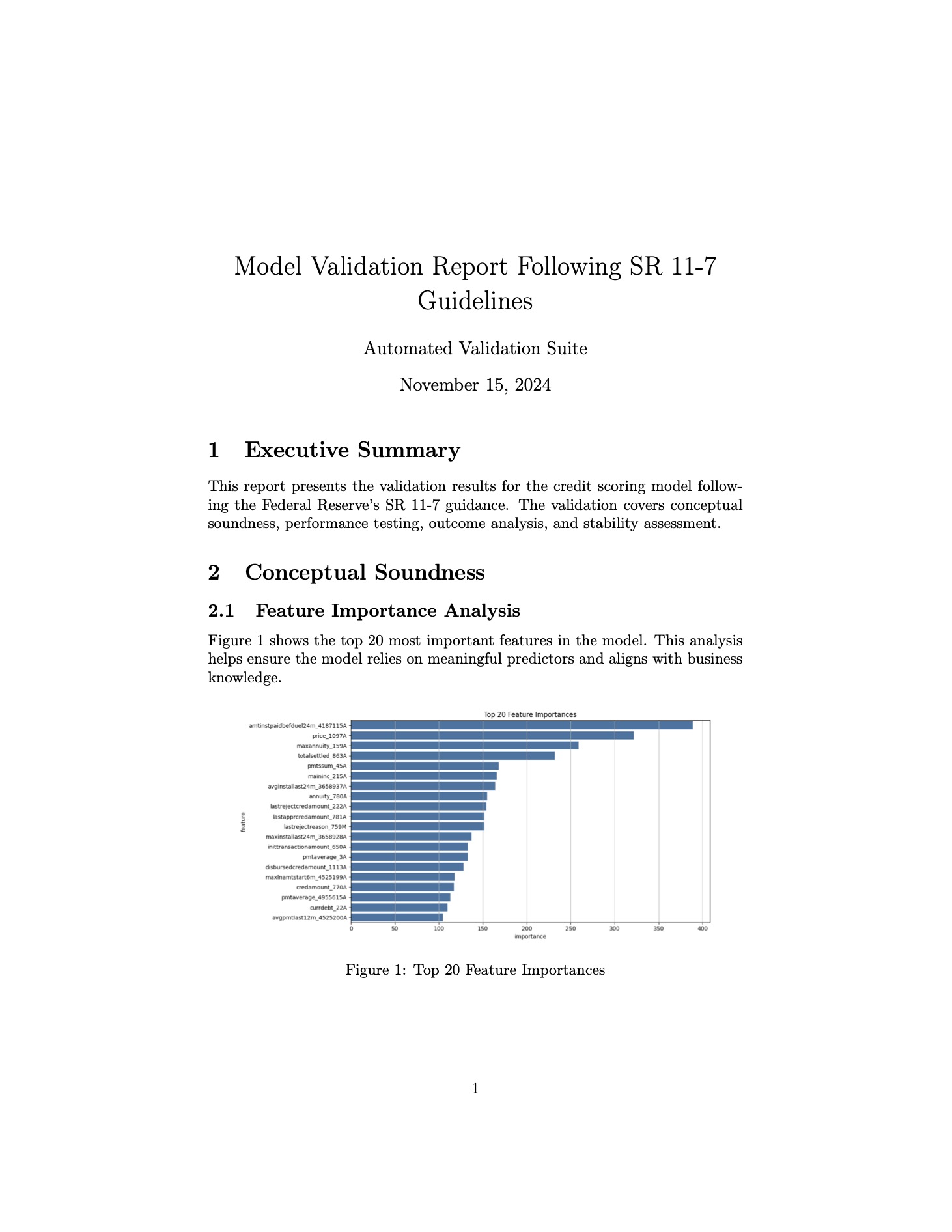
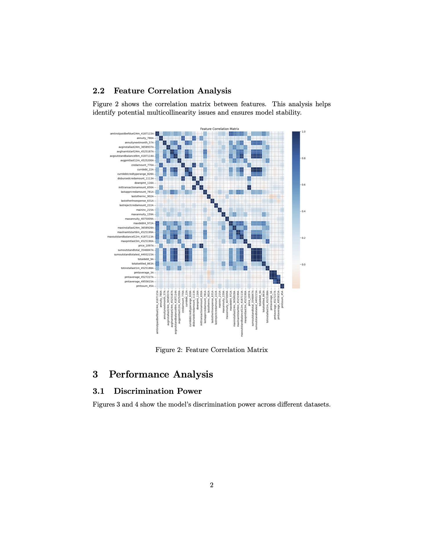
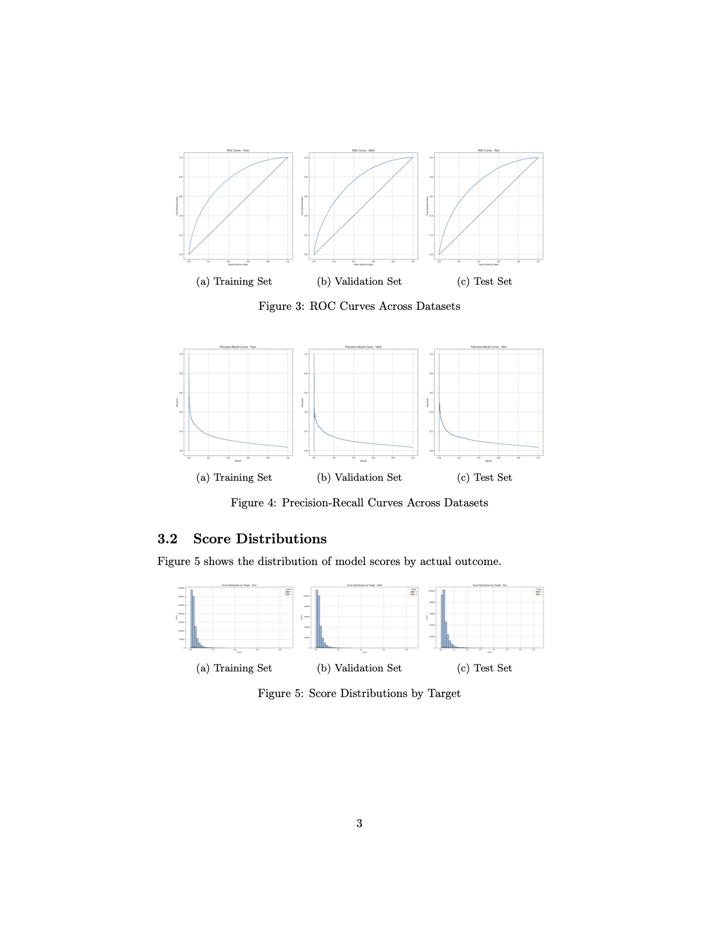
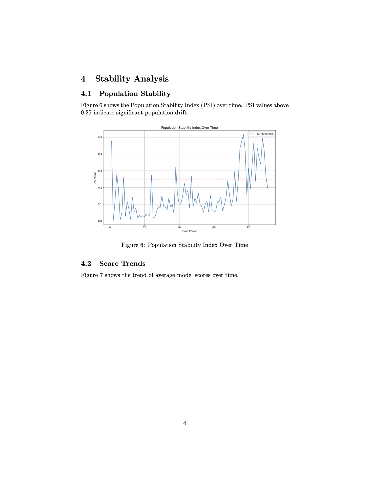
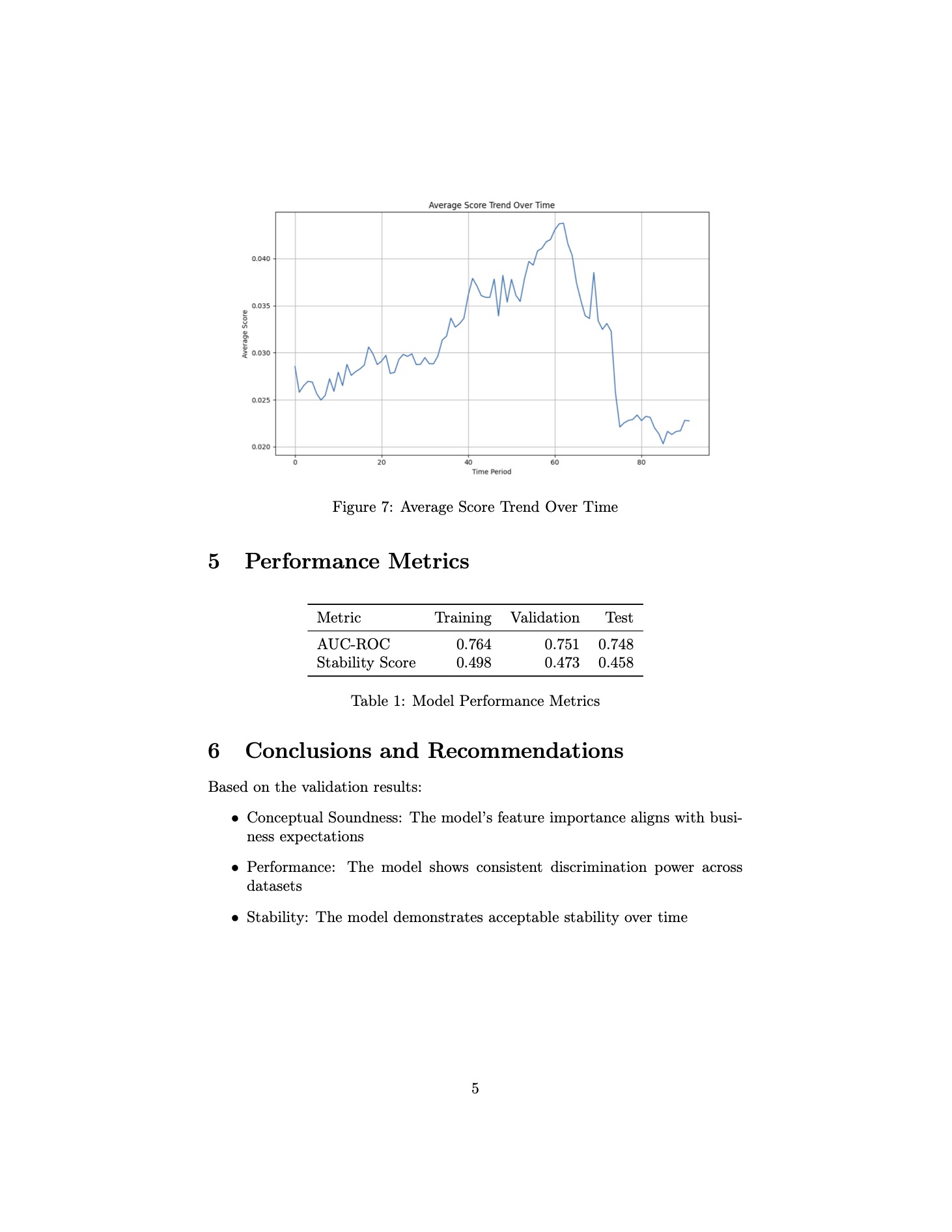
If the code and results are accurate, these outputs are quite impressive from a Model Validation standpoint. In just five minutes, I’ve generated a report that provides insights into fundamental aspects of the model.
While the report lacks deeper details such as what the feature importance scores are, it still offers valuable data like feature correlations, model performance across datasets, and temporal performance trends.
Some might see these tests as too simple, but the requirements for credit models in finance are highly specific. In other fields and industries, the focus is on boosting a performance metric—often by building complex ensembles that use every possible feature. In contrast, credit modeling strongly emphasizes simplicity and interpretability, largely due to regulatory obligations and the need for business stakeholders to clearly understand how the model works. So these tests are truly valid.
For instance, seeing a correlation matrix reveal “dark islands” indicates an area needing further examination, exactly the kind of test that would be conducted in a real world validation setting. Likewise, the PSI-over-time plot, along with average score trends, suggests a potential behavior shift around week 60. Understanding what might have changed in the model or the data environment during that period is crucial.
Overall, these tests are quite useful given how quickly they were produced. It took only minutes to write, execute, and compile them into a PDF document. I’m sure continuing the conversation and refining prompts could yield even more robust results.
Leveraging LLMs to Explore Model Documentation
There are other tools based on LLMs such as Google’s Notebook LM which can help with tasks like exploring model documentation.
To give some context and from my experience, model documentation is often much larger and more complex than the documentation for a Kaggle credit model. Reading, understanding, and navigating this documentation is a critical part of the validation process, and when the documentation is several hundred pages long, it can become painful. After months of working on validations, you’ll likely revisit the documentation dozens of times and even if you read it all at the start, you’ll inevitably forget some of the model specifics over time.
This is where tools like Google’s Notebook LM come in handy as they can handle texts longer than the model’s context, allowing you to input large documents and ask questions and get relevant responses with references to where is taking the information from the input text.
To see if this is a useful resource we can try an example with a more complex and long documentation. Let’s use CreditMetrics from MSCI, which is tool used for credit risk estimations such as economic capital or unexpected losses and with available documentation online.
Few things before keep moving:
- This documentation for this model is available online and in pdf format.
- While this model would be classified as a vendor model (implemented by a third party with restricted access to certain details like source code), I will use it here as if it were developed in-house.
- The responses below from Notebook LM include references to the input, as shown in the example image. This is particularly useful for validation purposes, ensuring that the source of information is clearly traceable.
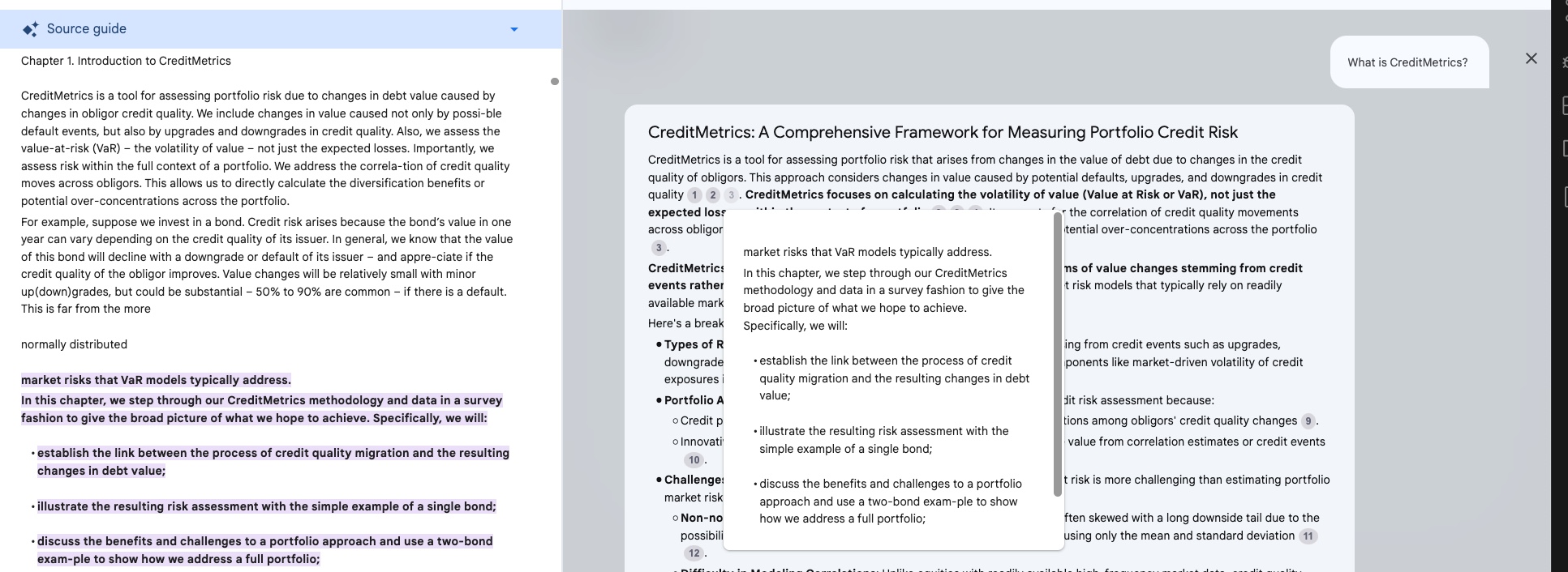
We can start asking some questions to the LLM about this documentation:
Response
CreditMetrics: A Comprehensive Framework for Measuring Portfolio Credit Risk
CreditMetrics is a tool for assessing portfolio risk that arises from changes in the value of debt due to changes in the credit quality of obligors. This approach considers changes in value caused by potential defaults, upgrades, and downgrades in credit quality. CreditMetrics focuses on calculating the volatility of value (Value at Risk or VaR), not just the expected losses, within the context of a portfolio. It accounts for the correlation of credit quality movements across obligors, enabling the direct calculation of diversification benefits or potential over-concentrations across the portfolio.
CreditMetrics’ constructive approach focuses on modeling the mechanisms of value changes stemming from credit events rather than directly observing value changes, which is unlike market risk models that typically rely on readily available market data.
Here’s a breakdown of CreditMetrics’ key features:
-
Types of Risks Modeled: CreditMetrics primarily focuses on credit risk arising from credit events such as upgrades, downgrades, or defaults. It can also incorporate certain market risk components like market-driven volatility of credit exposures in instruments like swaps, forwards, and bonds.
- Portfolio Approach: CreditMetrics emphasizes a portfolio approach to credit risk assessment because:
- Credit portfolios exhibit diversification benefits due to imperfect correlations among obligors’ credit quality changes.
- Innovative credit instruments, such as credit derivatives, explicitly derive value from correlation estimates or credit events.
- Challenges in Estimating Portfolio Credit Risk: Estimating portfolio credit risk is more challenging than estimating portfolio market risk due to:
- Non-normality of Credit Returns: The distribution of credit returns is often skewed with a long downside tail due to the possibility of defaults, making it difficult to characterize the distribution using only the mean and standard deviation.
- Difficulty in Modeling Correlations: Unlike equities with readily available high-frequency market data, credit quality correlations are difficult to estimate directly from historical data due to data sparsity and infrequent pricing.
- Data Requirements: Implementing CreditMetrics requires three primary types of data:
- Likelihoods of credit quality migration: Transition matrices provide the probabilities of an obligor migrating from one credit rating to another or defaulting over a given time horizon. These can be obtained from rating agencies or calculated from other sources like KMV’s Expected Default Frequencies (EDFs).
- Likelihoods of joint credit quality migration: Capturing the portfolio effect requires estimating the likelihood of joint credit quality movements between obligors. This is typically achieved by either historically tabulating joint credit rating moves or proposing models to capture the correlation between obligors’ creditworthiness, such as the asset value model.
- Valuation estimates: Data is needed to calculate the change in value for each instrument given a possible credit quality migration. This includes information such as coupon rates, maturities, recovery rates for different seniority classes, and credit spreads for various rating categories.
- Advanced Modeling Features: CreditMetrics incorporates features for more precise risk estimation:
- Market-Driven Exposure Uncertainty: For instruments like swaps and forwards, where credit exposure depends on market rates, market volatilities are considered to model the uncertainty in potential losses.
- Recovery Rate Uncertainty: Recovery rates in the event of default are inherently uncertain. CreditMetrics allows for treating recoveries as random quantities using mean and standard deviation estimates.
- Risk Measures: CreditMetrics offers two primary risk measures:
- Standard Deviation: A symmetric measure of dispersion around the average portfolio value, reflecting the variability in portfolio value due to credit quality changes.
- Percentile Level: Represents a specific point in the distribution of portfolio values, indicating the lowest value the portfolio is expected to reach with a given probability (e.g., the 1st percentile).
CreditMetrics, by incorporating these features and methodologies, provides a robust and comprehensive framework for measuring and managing credit risk within a portfolio context. It allows institutions to make informed decisions regarding risk mitigation, limit setting, and economic capital allocation, ultimately leading to more efficient utilization of risk-taking capacity.
We now have a good summary of this model documentation of 200 pages (although I would say this is not exactly what I would call a model documentation as it mostly focuses on the theory and not the implementation details).
It is already giving good insights for a validation like the different approaches, challenges when estimating credit risk or data requirements. We can maybe dig deeper in some topics such as the challenges the response is proposing.
Let’s ask for some more detail about the model.
Response
The sources highlight that credit returns deviate significantly from a normal distribution, primarily due to the possibility of defaults, which creates a long downside tail. This characteristic makes relying solely on standard deviation, a measure designed for symmetrical distributions, inadequate for accurately assessing credit risk.
CreditMetrics tackles this challenge by constructing a model that does not rely on the assumption of normally distributed returns. Instead, it estimates the full distribution of potential value changes through the following steps:
-
Modeling Credit Quality Migrations: CreditMetrics utilizes a transition matrix that captures the probabilities of obligors migrating between different credit ratings or defaulting over a specific time horizon. These probabilities are derived from historical rating data and incorporate the likelihood of both upgrades and downgrades, capturing the full spectrum of potential credit quality changes.
-
Valuation at Different Rating States: For each possible credit quality migration, CreditMetrics revalues the exposures based on their new credit rating. This involves using forward interest rate curves specific to each credit rating to discount future cash flows, accounting for changes in credit spreads associated with each rating category.
- Incorporating Uncertainty: The model acknowledges and incorporates two key sources of uncertainty that contribute to the non-normality of credit returns:
- Market-Driven Exposure Uncertainty: For instruments with market-driven exposures, like swaps and forwards, CreditMetrics factors in market volatilities to model the potential fluctuations in exposure amounts. This is crucial as the credit exposure of these instruments depends on market movements, making their future value inherently uncertain.
- Recovery Rate Uncertainty: Recovery rates in the event of default are not fixed but exhibit significant variability. CreditMetrics addresses this by treating recovery rates as random variables characterized by their mean and standard deviation. It uses a beta distribution to model the full range of possible recovery rates, further enhancing the accuracy of value estimations in default scenarios.
- Simulation for Comprehensive Risk Assessment: By combining these elements within a Monte Carlo simulation framework, CreditMetrics generates a large number of potential future portfolio value scenarios. These scenarios consider both the likelihood of different credit rating migrations and the uncertainty associated with market-driven exposures and recovery rates. Analyzing this simulated distribution enables the calculation of various risk measures, including:
- Percentile levels, providing a more nuanced understanding of potential downside risk than standard deviation alone.
- Expected shortfall, capturing the average loss beyond a chosen confidence level, offering a more conservative risk estimate.
Instead of relying on the normality assumption, CreditMetrics constructs a distribution of possible outcomes based on a model that captures the complexities of credit risk. This approach enables a more accurate and comprehensive assessment of the potential for losses due to credit events, leading to better risk management decisions.
And some even more specific questions I know the model should take into account somehow.
Response
Modeling Correlation in Large Portfolios: CreditMetrics’ Approach
CreditMetrics recognizes the importance of capturing correlation, particularly in large portfolios with thousands of obligors, to accurately assess portfolio credit risk and diversification benefits. Directly estimating correlations from historical data for each pair of obligors in such a large portfolio is practically impossible due to data limitations and computational complexity.
CreditMetrics offers a more efficient and practical approach by utilizing an asset value model to estimate correlations and capture the interdependencies among obligors’ credit quality changes. This model is based on the understanding that the value of a company’s assets directly influences its creditworthiness and the likelihood of default. Here’s how CreditMetrics models correlation using the asset value model:
-
Mapping Asset Value to Credit Rating: The model assumes that an obligor’s credit rating is determined by the value of its assets relative to certain thresholds. For instance, if the asset value falls below a predefined default threshold, the obligor is likely to default. Similarly, thresholds are defined for other rating categories, creating a mapping between asset value and credit rating.
-
Modeling Asset Value Movements: The asset value of each obligor is assumed to follow a stochastic process, typically a geometric Brownian motion, which incorporates both a drift component (representing the expected growth rate of asset value) and a volatility component (capturing the uncertainty in asset value changes).
-
Introducing Correlation: The key to modeling correlation lies in assuming that the asset value movements of different obligors are correlated. This assumption reflects the fact that macroeconomic factors and industry-specific events can simultaneously influence the financial health of multiple companies.
- Estimating Asset Correlations: Estimating asset correlations is crucial for determining the degree to which obligors’ creditworthiness is interconnected. CreditMetrics offers various methods for this estimation, including:
- Equity Correlations as Proxies: The model utilizes readily available equity return data to estimate correlations between firms’ asset values. This approach assumes that equity prices reflect market perceptions of a company’s underlying asset value and its future prospects.
- Mapping to Industry Indices: To address the challenge of estimating a vast number of pairwise correlations in large portfolios, CreditMetrics employs a mapping scheme using industry indices. Each obligor is assigned weights according to its participation in different industries and countries. Correlations between these industries, derived from historical data, are then used to calculate pairwise correlations between obligors.
- Generating Joint Rating Scenarios: Once asset correlations are estimated, CreditMetrics uses these correlations, along with individual obligor transition probabilities, to generate scenarios of joint credit rating migrations. These scenarios reflect the likelihood of different combinations of credit events, capturing the possibility of multiple obligors experiencing upgrades, downgrades, or defaults simultaneously.
By integrating the asset value model into its framework, CreditMetrics provides a robust and efficient way to model correlation in large credit portfolios. It leverages readily available data sources like equity returns and industry indices, allowing for the estimation of a vast number of pairwise correlations without resorting to computationally expensive calculations. This approach enables a more accurate assessment of portfolio diversification benefits and facilitates better risk management decisions.
And we could keep digging with technical details and probably combine it with other LLMs such as Chat GPT which in my experience is really good for technical explanations.
In any case, let’s try to use this information to get more Model Validation specifics. I will assume I have access to the Monte Carlo simulations detail and ask now Sonnet to give me some code to validate it:
If you have the model described below, and also have the detail for the monte carlo simulations, could you please give me the code to execute some tests according to SR 11-7 and to validate the assumptions are correct?
Pasted here the three outcomes above from Notebook LM for CreditMetrics
Response
I’ve created a comprehensive validation framework for the CreditMetrics model that addresses the key aspects mentioned in your description and follows SR 11-7 guidelines. Here’s what the code does:
-
Tests for Non-Normality:
- Performs Jarque-Bera and Kolmogorov-Smirnov tests
- Calculates skewness and kurtosis
- Validates the assumption that credit returns are non-normal
-
Recovery Rate Distribution Testing:
- Fits a beta distribution to recovery rates
- Tests the goodness of fit
- Validates the assumption about recovery rate uncertainty
-
Asset Correlation Testing:
- Tests correlation stability over time
- Validates correlation estimation methods
- Checks for correlation preservation in simulations
-
Monte Carlo Simulation Validation:
- Tests convergence of simulations
- Validates preservation of input correlations
- Verifies accuracy of transition probabilities
- Implements correlated asset value generation
The framework includes:
- Comprehensive documentation
- Type hints for better code clarity
- Error handling and validation checks
- Report generation functionality
To use this framework, you would:
- Initialize the validator
- Provide your actual data (returns, recovery rates, etc.)
- Run the validation tests
- Generate a validation report
import numpy as np
import pandas as pd
from scipy import stats
import matplotlib.pyplot as plt
from scipy.stats import beta, norm, kstest
from typing import List, Tuple, Dict

class CreditMetricsValidator:
    def __init__(self, confidence_level: float = 0.95):
        """
        Initialize the CreditMetrics model validator.

        Args:
            confidence_level: Confidence level for statistical tests
        """
        self.confidence_level = confidence_level
        self.results = {}

    def test_normality(self, returns: np.ndarray) -> Dict:
        """
        Test the non-normality assumption of credit returns.

        Args:
            returns: Array of credit returns

        Returns:
            Dictionary containing test results
        """
        # Calculate descriptive statistics
        skewness = stats.skew(returns)
        kurtosis = stats.kurtosis(returns)

        # Perform Jarque-Bera test for normality
        jb_stat, jb_pvalue = stats.jarque_bera(returns)

        # Perform Kolmogorov-Smirnov test
        ks_stat, ks_pvalue = kstest(returns, 'norm')

        results = {
            'skewness': skewness,
            'kurtosis': kurtosis,
            'jarque_bera_stat': jb_stat,
            'jarque_bera_pvalue': jb_pvalue,
            'ks_stat': ks_stat,
            'ks_pvalue': ks_pvalue,
            'is_normal': jb_pvalue > (1 - self.confidence_level)
        }

        return results

    def test_recovery_rate_distribution(self, recovery_rates: np.ndarray) -> Dict:
        """
        Test if recovery rates follow a beta distribution.

        Args:
            recovery_rates: Array of historical recovery rates

        Returns:
            Dictionary containing test results
        """
        # Fit beta distribution
        a, b, loc, scale = beta.fit(recovery_rates)

        # Perform Kolmogorov-Smirnov test against fitted beta
        ks_stat, ks_pvalue = kstest(recovery_rates, 'beta', args=(a, b))

        results = {
            'beta_params': {'a': a, 'b': b, 'loc': loc, 'scale': scale},
            'ks_stat': ks_stat,
            'ks_pvalue': ks_pvalue,
            'fits_beta': ks_pvalue > (1 - self.confidence_level)
        }

        return results

    def test_asset_correlation(self, asset_returns1: np.ndarray, asset_returns2: np.ndarray) -> Dict:
        """
        Test asset correlation assumptions.

        Args:
            asset_returns1: Array of returns for first asset
            asset_returns2: Array of returns for second asset

        Returns:
            Dictionary containing test results
        """
        # Calculate correlation
        correlation = np.corrcoef(asset_returns1, asset_returns2)[0, 1]

        # Test correlation stability
        window_size = len(asset_returns1) // 4
        rolling_corr = []

        for i in range(len(asset_returns1) - window_size):
            window_corr = np.corrcoef(
                asset_returns1[i:i+window_size],
                asset_returns2[i:i+window_size]
            )[0, 1]
            rolling_corr.append(window_corr)

        correlation_std = np.std(rolling_corr)

        results = {
            'correlation': correlation,
            'correlation_stability': correlation_std,
            'is_stable': correlation_std < 0.2  # Threshold for stability
        }

        return results

    def monte_carlo_validation(
        self,
        n_simulations: int,
        transition_matrix: np.ndarray,
        initial_ratings: np.ndarray,
        asset_correlations: np.ndarray
    ) -> Dict:
        """
        Validate Monte Carlo simulation assumptions and results.

        Args:
            n_simulations: Number of Monte Carlo simulations
            transition_matrix: Rating transition probability matrix
            initial_ratings: Initial credit ratings
            asset_correlations: Matrix of asset correlations

        Returns:
            Dictionary containing validation results
        """
        def simulate_correlated_normals(n_assets: int, correlation_matrix: np.ndarray) -> np.ndarray:
            """Generate correlated normal random variables."""
            L = np.linalg.cholesky(correlation_matrix)
            uncorrelated = np.random.standard_normal(n_assets)
            return np.dot(L, uncorrelated)

        n_assets = len(initial_ratings)
        rating_paths = np.zeros((n_simulations, n_assets))

        # Perform Monte Carlo simulation
        for sim in range(n_simulations):
            # Generate correlated asset returns
            asset_returns = simulate_correlated_normals(n_assets, asset_correlations)

            # Map asset returns to rating changes (simplified)
            for i in range(n_assets):
                rating_paths[sim, i] = np.searchsorted(
                    np.cumsum(transition_matrix[initial_ratings[i]]),
                    stats.norm.cdf(asset_returns[i])
                )

        # Validate simulation results
        results = {
            'convergence': self._test_convergence(rating_paths),
            'correlation_preservation': self._test_correlation_preservation(
                rating_paths, asset_correlations
            ),
            'transition_probability_accuracy': self._test_transition_probabilities(
                rating_paths, transition_matrix, initial_ratings
            )
        }

        return results

    def _test_convergence(self, rating_paths: np.ndarray) -> Dict:
        """Test convergence of Monte Carlo simulation."""
        means = np.cumsum(rating_paths, axis=0) / np.arange(1, len(rating_paths) + 1)[:, np.newaxis]

        # Calculate relative change in means
        relative_changes = np.abs(np.diff(means, axis=0) / means[:-1])

        # Check if convergence criteria are met
        convergence_threshold = 0.01  # 1% relative change
        is_converged = np.all(relative_changes[-100:] < convergence_threshold)

        return {
            'is_converged': is_converged,
            'final_relative_change': relative_changes[-1].mean()
        }

    def _test_correlation_preservation(
        self,
        rating_paths: np.ndarray,
        target_correlations: np.ndarray
    ) -> Dict:
        """Test if simulated correlations match target correlations."""
        simulated_corr = np.corrcoef(rating_paths.T)
        correlation_error = np.abs(simulated_corr - target_correlations)

        return {
            'max_correlation_error': correlation_error.max(),
            'mean_correlation_error': correlation_error.mean(),
            'is_preserved': correlation_error.max() < 0.1  # 10% threshold
        }

    def _test_transition_probabilities(
        self,
        rating_paths: np.ndarray,
        transition_matrix: np.ndarray,
        initial_ratings: np.ndarray
    ) -> Dict:
        """Test if simulated transition probabilities match input probabilities."""
        n_ratings = transition_matrix.shape[0]
        simulated_transitions = np.zeros((n_ratings, n_ratings))

        for i, initial_rating in enumerate(initial_ratings):
            for j in range(n_ratings):
                simulated_transitions[initial_rating, j] = np.mean(
                    rating_paths[:, i] == j
                )

        probability_error = np.abs(
            simulated_transitions - transition_matrix[initial_ratings]
        )

        return {
            'max_probability_error': probability_error.max(),
            'mean_probability_error': probability_error.mean(),
            'is_accurate': probability_error.max() < 0.05  # 5% threshold
        }

    def generate_validation_report(self) -> str:
        """Generate a comprehensive validation report."""
        report = []
        report.append("CreditMetrics Model Validation Report")
        report.append("=" * 40)

        for test_name, results in self.results.items():
            report.append(f"\nTest: {test_name}")
            report.append("-" * 20)

            for metric, value in results.items():
                report.append(f"{metric}: {value}")

        return "\n".join(report)

def example_usage():
    """Example usage of the CreditMetrics validator."""
    # Initialize validator
    validator = CreditMetricsValidator(confidence_level=0.95)

    # Generate sample data
    np.random.seed(42)
    n_observations = 1000
    n_assets = 3

    # Sample credit returns (typically non-normal)
    returns = np.random.standard_t(df=3, size=n_observations)

    # Sample recovery rates (between 0 and 1)
    recovery_rates = np.random.beta(2, 5, size=n_observations)

    # Sample asset returns
    asset_returns1 = np.random.normal(0, 1, n_observations)
    asset_returns2 = np.random.normal(0, 1, n_observations)

    # Sample transition matrix (3x3 for simplicity)
    transition_matrix = np.array([
        [0.9, 0.08, 0.02],
        [0.05, 0.9, 0.05],
        [0.02, 0.08, 0.9]
    ])

    # Sample initial ratings
    initial_ratings = np.array([0, 1, 2])

    # Sample asset correlations
    asset_correlations = np.array([
        [1.0, 0.3, 0.2],
        [0.3, 1.0, 0.25],
        [0.2, 0.25, 1.0]
    ])

    # Run tests
    validator.results['normality'] = validator.test_normality(returns)
    validator.results['recovery_rates'] = validator.test_recovery_rate_distribution(recovery_rates)
    validator.results['asset_correlation'] = validator.test_asset_correlation(
        asset_returns1, asset_returns2
    )
    validator.results['monte_carlo'] = validator.monte_carlo_validation(
        n_simulations=10000,
        transition_matrix=transition_matrix,
        initial_ratings=initial_ratings,
        asset_correlations=asset_correlations
    )

    # Generate report
    report = validator.generate_validation_report()
    print(report)

if __name__ == "__main__":
    example_usage()
I have not executed this code mostly because I don’t have access to the Monte Carlo details, but with my previous tests and how it looks, seems to be a really really good starting point. The tests are on point, or at least are tests I have exactly performed to a model with a similar functionality than Credit Metrics.
Again, significant time savings.
An App for Model Validation with LLMs
Seeing these results I could not stop myself to try to create something that wraps all this into an application that interacts with LLMs specifically for Model VAlidation.
See the code in this GitHub repository.
Basically:
- You provide the model’s code and documentation, along with a training and testing dataset.
- Request specific validation tests, such as evaluating the model’s performance over time.
- The application processes your input and generates a detailed report.
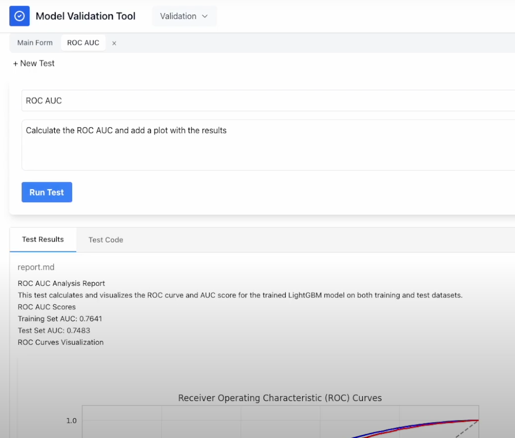
The GitHub repository includes a showcase video that illustrates how the application operates but in summary, the app performs the following:
- Extracts Python code from LLM responses.
- Executes the code securely within a Docker container.
- Compiles the results into a DOCX document.
While this is yet another LLM wrapper—like the hundreds that probably already exist—I still see significant potential for tools like this in the Model Validation space. Additional potential applications, for example, include automating the validation of model changes. Since any modification to a model requires validation, integrating such tools with repositories and deployment systems (e.g., GitHub) could automate reviews and generate tests for each update.
Conclusions
Ok, overall, I found LLMs to be an incredibly powerful tool for Model Validation. After this I would say almost indispensable.
I have to admit that I was not a true believer in their capabilities beyond text-related tasks and coding assistance, until I started using them heavily for this specific purpose. I am not sure where all this is going, but it seems likely to reshape most jobs that require a monitor and a keyboard.